Error Scaling Under Refinement
Here, we present extended measurements of the value function error scaling under grid refinement, as well as error maps showing where in state space this error is concentrated. The setup of our test cases on this page mirrors that of the Examples page. To estimate the error, we label "ground truth" \(v^\ast(\boldsymbol{r}, q)\) as the numerical solution on an extremely fine grid \( (N_r, N_\theta) = (3202, 4024) \). We then measure how the numerical solution on coarser grids deviates from this ground truth on the gridpoints that they share.
Error Scaling
Here, we present how the errors of our two adaptive time discretizations decrease when we increase the granularity of the state space grid mesh. In the "standard" discretization, we choose timesteps at each point in state space as \( \tau = 1.5\min(\Delta r / \dot{r}(r, \theta, q, u), \Delta \theta / \dot{\theta}(r, \theta, q, u)) \). In the nearly-causal "row-wise" discretization, we choose \( \tau = 1.5\Delta r / \dot{r}(r, \theta, q, u) \).
L1 Errors
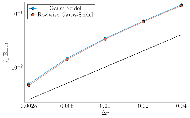
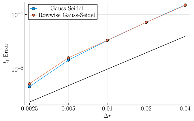
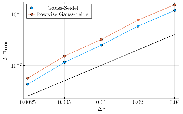
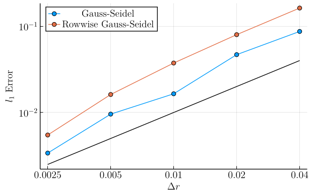
In the first set of plots, we show the mean \(l_1\)-error \(\left(\frac{1}{N_{\mathrm{pts}}} \sum_{\boldsymbol{r}, q}|v(\boldsymbol{r}, q) - v^\ast(\boldsymbol{r}, q)|\right)\) as a function of grid refinement. In these plots, the solid black line is simply a linear function chosen to compare these curves to slope-\(1\) in log-log space, showing that the mean \(l_1\) error in both methods decays roughly linearly with the grid cell lengths.
Here, we see that on the state space as a whole, our row-wise discretization is not causing dramatic changes in the error. In particular, at low drift constants, the error curves are nearly identical. However, a small gap between the two discretizations does appear with increasing drift strength.
Example 1 (Fully Deterministic):
- \(\sigma = 0.0\)
- \(a = 0.0\)
Example 2 (Moderate Diffusion, Zero Drift):
- \(\sigma = 0.1\)
- \(a = 0.0\)
Example 3 (Weak Diffusion, Weak Drift):
- \(\sigma = 0.05\)
- \(a = 0.05\)
Example 4 (Weak Diffusion, Strong Drift):
- \(\sigma = 0.05\)
- \(a = 0.15\)
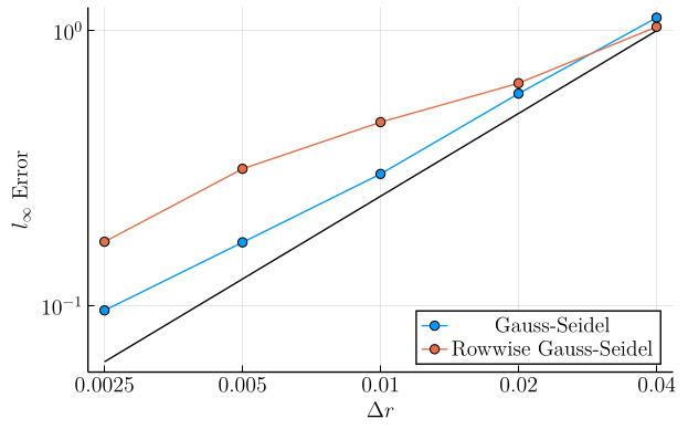
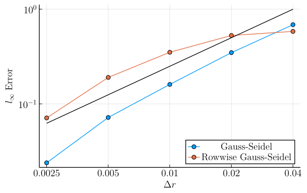
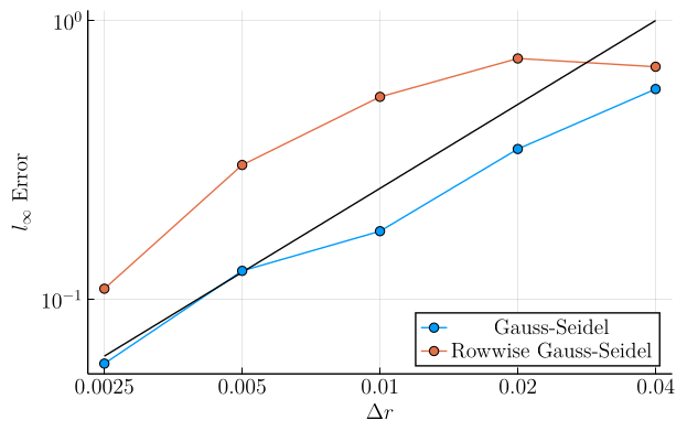
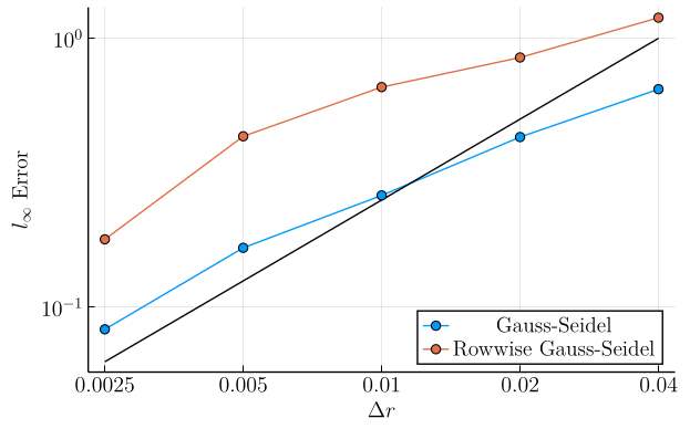
L∞ Errors
In this second set of plots, we show the \(l_\infty\)-error \(\left( \max_{\boldsymbol{r}, q} |v(\boldsymbol{r}, q) - v^\ast(\boldsymbol{r}, q)|\right)\) as a function of grid refinement. In these plots, the solid black line is simply a linear function chosen to compare these curves to slope-\(1\) in log-log space, showing that the \(l_\infty\) error in both methods decays roughly linearly with the grid cell lengths for fine grid meshes.
These plots show that, while our new discretization is generally accurate on most the domain, we can develop some "hot spots" whose error does not decay as quickly, particularly at low grid mesh sizes. However, at fine grid mesh sizes we appear to be re-attaining similar scaling between the two approaches.
Example 1 (Fully Deterministic):
- \(\sigma = 0.0\)
- \(a = 0.0\)
Example 2 (Moderate Diffusion, Zero Drift):
- \(\sigma = 0.1\)
- \(a = 0.0\)
Example 3 (Weak Diffusion, Weak Drift):
- \(\sigma = 0.05\)
- \(a = 0.05\)
Example 4 (Weak Diffusion, Strong Drift):
- \(\sigma = 0.05\)
- \(a = 0.15\)
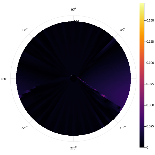
Error Maps
We have seen how the error of both methods decreases roughly similarly with increasing mesh granularity. Here, we present maps which show how this error is distributed in state space for the row-wise Gauss-Seidel iteration, showing the pointwise absolute error of the second-finest grid mesh \((N_r, N_\theta) = (1601, 2012)\) relative to the finest. Note that we are only showing the error map of a single tack (\(q = 1\)) here.
Example 1 (Fully Deterministic):
- \(\sigma = 0.0\)
- \(a = 0.0\)
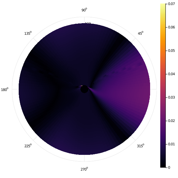
Example 2 (Moderate Diffusion, Zero Drift):
- \(\sigma = 0.1\)
- \(a = 0.0\)
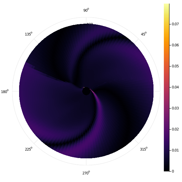
Example 3 (Weak Diffusion, Weak Drift):
- \(\sigma = 0.05\)
- \(a = 0.05\)
Example 4 (Weak Diffusion, Strong Drift):
- \(\sigma = 0.05\)
- \(a = 0.15\)
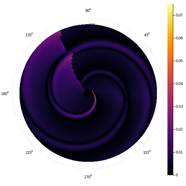
In particular, we clearly see that the errors in the "row-wise Gauss-Seidel" discretization are heavily concentrated immediately adjacent to the target in state space. Even more specifically, we notice two "hot spots" which seems to have far worse error that the rest of state space. The high-error zones in the rest of state space can be seen to "spiral" out from these hot spots that they are causally linked to.
Manually inspecting the scenario at this point, we find that these hot spots occur when the optimal trajectory is for the sailboat to approach the target very nearly tangentially to avoid a switching cost. In this case, our row-wise approach will pick extremely large timestep discretizations and choices between different control angles \(u\) change the value function greatly.