Planning During the Yellow, Red, and Green Phases

These supplemental movies and figures correspond to Example 3 of the following paper:

Planning During the Yellow, Red, and Green Phases:

Planning begins at \(t = T_Y\).
Driver knows \(T_Y\), \(T_R\) and \(T_G\) with certainty.
Yellow light duration, \(D_Y = 3s\).
Red light duration, \(D_R = 60s\).
Objective preferences: \((c_1,c_2,c_3) = (1/3, 1/3, 1/3)\).

In all figures, the white region appearing in the domain corresponds to illegal \((d,v)\) configurations belonging to \(\mathcal{I}_Y(t)\). As \(t \rightarrow T_R\), \(\mathcal{I}_Y(t) \rightarrow \mathcal{I}_R(t)\).

Feedback Controls and Trajectory Tracing:

Traces two optimal trajectories starting from \((d,v) = (d_0, v_0)\).
Black circle: \((d_0, v_0)\) = \((43, 10)\).
White circle: \((d_0, v_0)\) = \((48, 10)\).
\(t = 0\) in the animation corresponds to \(t = T_Y\).

Value Function Contour Plotting:

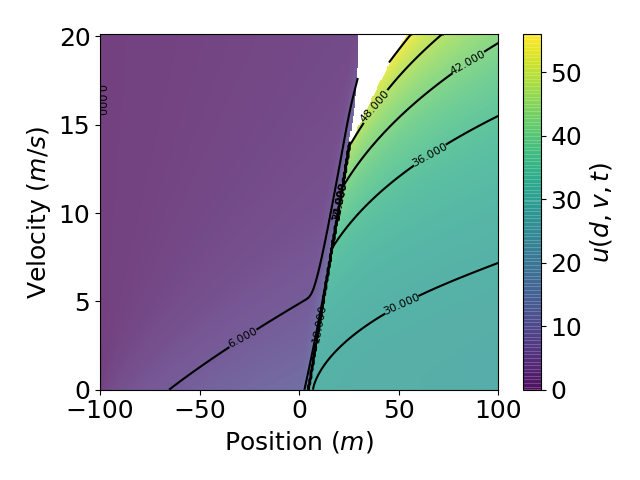
This section displays two snapshots of the value function contours during the yellow-light phase.

\(u(d,v,t) = + \infty\) at all \((d,v) \in \mathcal{I}_Y(t)\)

\(u(d,v,t)\) at \(t = T_Y\):

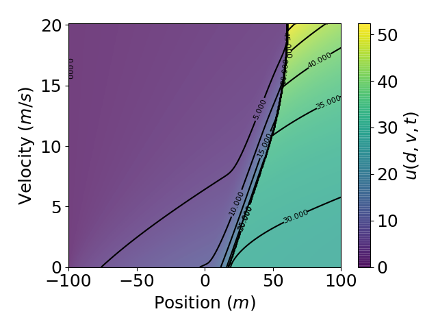
\(u(d,v,t)\) at \(t = T_Y + 1.5s\):

« Red Phase Planning Uncertain Green Phase Planning »